A Complete Worked Example: Lionepha
(Software Prerequisites)
For this exercise, in addition to DELINEATE you will need the following programs installed on your execution host:
For meta-analysis and visualization, you should have the following installed on your local machine:
In addition, of course (as always, for anything and everything), you will want a *good* text editor.
(Data Files)
All data files for this exercise are available for download here:
Introduction
We are going to to carry out a full species delimitation analysis, or, actually, a series of species delimitation analyses. We are going to use the the Lionepha system, using a subset of the data published by David R. Maddison and John S. Sproul:
David R Maddison, John S Sproul. Species delimitation, classical taxonomy and genome skimming: a review of the ground beetle genus Lionepha (Coleoptera: Carabidae), Zoological Journal of the Linnean Society, , zlz167, https://doi.org/10.1093/zoolinnean/zlz167.
The original data is available in the following Dryad repository:
The work by Maddison and Sproul (2020) nicely lays out the basic alpha taxonomy of this system, organizing these 143 lineages into 12 nominal species. This alpha taxonomy is based on a thorough analyses integrating morphological as well as genomic information, and thus we already have a very clear understanding of the species boundaries in this group, precluding the need for a species delimitation analysis.
However, for the purposes of this exercise we are going to pretend that this is not the case. Instead, we are going to consider that while the species identities of some of the population lineages are well known, in this sample there are number of lineages for which this is not the case.
Background
Study Design
We can imagine our study sampled individuals from an extensive range of localities, supplementing it with samples from previous collections, to develop a comprehensive data set spanning a broad taxonomic as well as geographic range. Preliminary phylogenetic analysis, which included genomic data from known, stable, species, as well as comparative morphological analyses, has confidentally established the species identities of some of these lineages. However, a number of lineages in the sample, while coming out to sister to known species, are sufficiently different in some respects (e.g., genetic distance or morphology), to make us question whether or not we are looking at different populations of the same species or perhaps new species altogether.
Alternatively, we might imagine a study to delineate species units in a particularly problematic clade. Here, in addition to samples from multiple populations from the clade, we would also include populations from a broader range of species in which the focal clade is a nested subtree. The analytical workflow for this sort of study will be identical to that discussed here, with only the distribution of population lineages of unknown identity being different — clustered into a single subtree on the larger phylogeny as opposed to scattered into multiple smaller subtrees (or single lineages).
Data
Here we will focus on just a subset of the data from Maddison and Sproul (2020), focusing only on lineages in the genus Lionepha itself. This data consists of 8 gene alignments for 143 samples from multiple individuals from multiple populations from multiple species:
lionepha/00-alignments/18s.nex
lionepha/00-alignments/28s.nex
lionepha/00-alignments/argk.nex
lionepha/00-alignments/cad.nex
lionepha/00-alignments/coi.nex
lionepha/00-alignments/msp.nex
lionepha/00-alignments/topo.nex
lionepha/00-alignments/wg.nex
Stage I: Identification of Population Units using the Multipopulation Coalescent Model
The first stage of our analysis will be delimitation of population units, i.e. assignment of population identities to individual lineages, under the “multipopulation coalescent”. This model was first published under the name “censored coalescent”, but has since become more popularly known as the “Multispecies Coalescent” or “MSC” model. It is a very powerful and elegant model that allows us to identify structure in genomic data arising from disruptions in Wright-Fisher panmixia due to restrictions in gene flow.
We will be using BP&P to identify our population units, and StarBeast2 to obtain a guide tree for the BP&P analysis. Note that these programs use the term “species” to reference the higher-level units they analyze rather than populations (as in “species delimitation” or “species tree inference”, rather than “population delimitation” and “population tree inference”). This can be correct in some contexts: e.g., where the data sampling does, either coincidentally or by design, indeed represent a 1-to-1 correspondence between populations and species, or, equivalently the species being studied do indeed not have any within-species lineage structure. However, more generally, this is, at best, misleading. These programs use the MSC as their underlying model. From a statistical perspective, it is uncontroversial that the biological units that these programs model through the “censored” coalescent/MSC that model that underlies them are (Wright-Fisher) populations. Strictly speaking, when used for species delimitation or model species trees, programs such as BP&P and StarBeast2 are used to identify population units under the MSC, and then these population units are interpreted (with or without justification) by the investigator to correspond on a 1-to-1 basis to species units. Thus, when using the MSC for “species delimitation” or “species tree inference”, the difference between “population” and “species” is purely lexical rather than statistical.
Here, however, we are going to interpret higher-level units of organization as exactly what they are as modeled by the MSC — populations, no more and no less. Unfortunately, this may result in some confusion as both BP&P and StarBeast2 refer to the higher-level units they target as “species” at least some of the time in the various program options and documentation. (In fact, BP&P, in some of the program documentation as well as n some of the various papers presenting or referencing the theory behind it acutally use the term “species” and “populations” interchangeably). This is simply the cost of doing business.
Candidate Population Units
A BP&P analysis requires us to identify “population” lineages as input a priori, some of which it will then collapse together to form “species” lineages. As we have noted (and as we will note again!), this terminological choice is not generally correct (it may apply in some special cases, such as single-population species systems, single-population-sample-per-species datasets, or where the data are too weak to detect population structure). We will instead consider these to be “candidate population” and “actual population” lineages respectively. That is, we will provide BP&P with the finest-grain units that could possibly be distinct populations as candidate population lineages, then use the power of the MSC model to accurately merge together our candidate populations into distinct populations (“species”, in BP&P terminology). For this analysis, we will err on the side of caution, not hestitating our over-split our candidate populations, as we can rely on the MSC to collapse them if there is insufficient gene flow restriction between them to form population boundaries. As such, we will consider every distinct geographical sample to be a distinct candidate population.
Individual |
Candidate Population Assignment |
|---|---|
|
L_australerasa_CA_Carson_Spur |
|
L_australerasa_CA_Homewood_Canyon |
|
L_australerasa_CA_Martin_Meadow |
|
L_australerasa_CA_Mill_Creek |
|
L_australerasa_CA_Nanny_Creek |
|
L_australerasa_CA_Oyster_Lake |
|
L_australerasa_OR_Crater_Lake |
|
L_casta_AK_Ketchikan |
|
L_casta_AK_Prince_of_Wales_Island |
|
L_casta_CA_Mt_Tamalpais |
|
L_casta_CA_Soda_Creek |
|
L_casta_CA_West_Branch_Mill_Creek |
|
L_casta_OR_Lost_Prairie |
|
L_casta_OR_Marys_Peak |
|
L_casta_OR_School_Creek |
|
L_casta_WA_Taneum_Creek |
|
L_disjuncta_BC_Summit_Creek |
|
L_disjuncta_CA_Emerson_Creek |
|
L_disjuncta_CA_Lily_Lake |
|
L_disjuncta_CA_Salmon_Creek |
|
L_disjuncta_CA_Trinity_Alps |
|
L_disjuncta_ID_Salmon_River |
|
L_disjuncta_MT_Mill_Creek |
|
L_disjuncta_OR_Lostine_River |
|
L_disjuncta_OR_Mt_Hood |
|
L_erasa_AK_Thompson_Pass |
|
L_erasa_BC_Cherryville |
|
L_erasa_OR_Lost_Prairie |
|
L_erasa_OR_Marys_Peak |
|
L_erasa_OR_Mount_Hebo |
|
L_erasa_OR_Mt_Hood |
|
L_erasa_OR_Prairie_Peak |
|
L_kavanaughi_MT_Bitterroot_River |
|
L_kavanaughi_MT_Lost_Horse_Creek |
|
L_kavanaughi_OR_Little_Philips_Creek |
|
L_kavanaughi_OR_Lostine_River |
|
L_kavanaughi_OR_Lostine_River_Valley |
|
L_lindrothi_CA_Deadman_Creek |
|
L_lindrothi_CA_East_Fork_Kaweah_River |
|
L_lindrothi_CA_Emerald_Lake |
|
L_lindrothi_CA_Kaiser_Pass |
|
L_lindrothi_CA_Long_Valley_Creek |
|
L_lindrothi_CA_Sonora_Pass |
|
L_lindrothi_CA_South_Fork_Bishop_Creek |
|
L_lindrothi_CA_Tioga_Lake |
|
L_osculans_CA_Carson_Spur |
|
L_osculans_CA_Cold_Creek |
|
L_osculans_CA_Los_Padres_NF |
|
L_osculans_CA_Nanny_Creek |
|
L_osculans_CA_Pike_County_Gulch |
|
L_osculans_CA_Rainbow |
|
L_osculans_CA_Stanislaus_NF |
|
L_osculans_CA_Strawberry_Creek |
|
L_osculans_CA_Warner_Range |
|
L_osculans_OR_Eugene |
|
L_osculans_OR_Goodman_Creek |
|
L_osculans_OR_Little_Philips_Creek |
|
L_osculans_OR_Middle_Fork_Berry_Creek |
|
L_osculans_OR_School_Creek |
|
L_osculans_OR_Walton_Lake |
|
L_probata_BC_Summit_Creek |
|
L_probata_CA_Algoma_Camp |
|
L_probata_CA_Ellery_Lake |
|
L_probata_CA_Middle_Martis_Creek |
|
L_probata_CA_Nanny_Creek |
|
L_probata_CA_Sherman_Pass |
|
L_probata_CA_South_Fork_Bishop_Creek |
|
L_probata_CA_Squaw_Valley_Resort |
|
L_probata_CA_Strawberry_Creek |
|
L_probata_CA_Tamarack_Lake |
|
L_probata_CA_Warner_Range |
|
L_probata_CA_White_Mountains |
|
L_probata_ID_Baker_Creek |
|
L_probata_ID_Galena_Summit |
|
L_probata_ID_Park_Creek |
|
L_probata_MT_Mill_Creek |
|
L_probata_MT_Prospect_Creek |
|
L_probata_NV_Ruby_Mountains |
|
L_probata_OR_Little_Philips_Creek |
|
L_probata_OR_Lonesome_Spring |
|
L_probata_OR_Lost_Prairie |
|
L_probata_OR_Lostine_River_Valley |
|
L_probata_OR_Lostine_River_Valley |
|
L_probata_OR_Mt_Ashland |
|
L_probata_OR_Odell_Creek |
|
L_probata_OR_Steens_Mountains |
|
L_probata_UT_Shingle_Creek |
|
L_probata_UT_Stansbury_Mtns |
|
L_probata_UT_Tushar_Mountains |
|
L_probata_WA_Blue_Mountains |
|
L_probata_WA_Taneum_Creek |
|
L_pseudoerasa_CA_Kaiser_Pass |
|
L_pseudoerasa_CA_Lily_Lake |
|
L_pseudoerasa_CA_Sherman_Pass |
|
L_pseudoerasa_CA_Strawberry_Creek |
|
L_pseudoerasa_CA_Trinity_Alps |
|
L_sequoiae_CA_Bridal_Veil_Falls |
|
L_sequoiae_CA_Nanny_Creek |
|
L_sequoiae_CA_Strawberry_Creek |
|
L_sequoiae_OR_Oakridge |
|
L_sequoiae_OR_School_Creek |
|
L_tuulukwa_CA_Trinity_Alps |
|
L_tuulukwa_OR_Knowles_Creek |
|
L_tuulukwa_OR_Marys_Peak |
Generating a Guide Tree for Population Delimitation
We will provide BP&P with a guide tree for its population delimitation analysis. We will use StarBeast2 to generate this guide tree.
The full StarBeast2 configuration file, generated using BEAUTi, can be found at in lionepha/01-guidetree-estimation/sb00500M.xml.
The alignments listed above were imported, and the following “traits” file was used to map alignment sequences to canidate population units: lionepha/01-guidetree-estimation/traits.txt.
We used a single strict clock model across all genes, and a HKY+G model of substitution.
We ran four replicates of this analysis for 500 million generations each, sampling every 500,000 generations for a total of 1000 samples from each replicates. The first 250 samples were discarded from the 100 samples of each replicates. Convergence was diagnosed through inspection of traces for each parameter as well as the likelihood and posterior. ESS values for each parameter were established to be more than 250, and distributions of parameter values were compared to a “null” run (i.e., a run without data where just the prior was sampled) to confirm that the analysis learned from the data sufficiently to shift the posterior away from the prior.
The post-burn in samples from the posterior were summarized using SumTrees, with the following command:
$ sumtrees.py -b 250 \
            -s mcct \
            -e clear \
            -l clear \
            --force-rooted \
            --suppress-annotations \
            -r -o summary.guide.tre \
            run1/species.trees \
            run2/species.trees \
            run3/species.trees \
            run4/species.trees
This selects the Maximum Clade Credibility Tree (MCCT) tree for the summary topolgy, stripping all branch lengths and metadata annotations, to result in the following:
lionepha/01-guidetree-estimation/guidetree.nex
Delimitation of Population Units
Now that we have a guide tree that treats each distinct geographical lineage as a candidate distinct Wright-Fisher population, we will run BP&P in “A10” mode to delimit the true population units under the “multipopulation coalescent” (i.e., the MSC).
For Small Datasets: the Single-Analysis Approach
The files provided in the lionepha/02a-population-delimitation-pooled directory set up a fairly straightforward BP&P “A10” analyses using the data that we have collected and the guide tree we have estimated:
File |
Description |
|---|---|
bpprun.input.ctl |
Control file |
bpprun.input.chars.txt |
Character data |
bpprun.input.imap.txt |
Sequence to population map |
bpp00.job |
Execution job |
The problem is that, when executing the analysis by either running the job file:
$ bash bpp00.job
or submitting it to an execution host:
$ qsub bpp00.job
or simply running the command directly:
$ bpp --cfile bpprun.input.ctl
we might find that the data set is too large to analyze:
bpp v4.1.4_linux_x86_64, 31GB RAM, 12 cores
https://github.com/bpp
.
.
.
Total species delimitations: 23958541050464777
Unable to allocate enough memory.
For Larger Datasets: the Subtree Decomposition Approach
The solution is to break the data set up into subtrees and carry out a separate population delimitation analysis on each subtree. While designing a decomposition scheme, it is important to note that we should not separate out candidate population lineages that might potentially belong to the same (actual) population into separate subtrees, thereby preventing BP&P from being able to collapse them if it does not detect any gene flow restriction between them. In most studies, this should not be too difficult to identify. Even in cases where we might not know where the species boundaries are, with reference to the guide tree phylogeny we should be able to identify subtree clusters that do not disrupt population boundaries. In this case of this Lionepha study, the nominal species clades provide very nice granularity — small enough to be analyzed by BP&P, yet with no danger of breaking up an actual population.
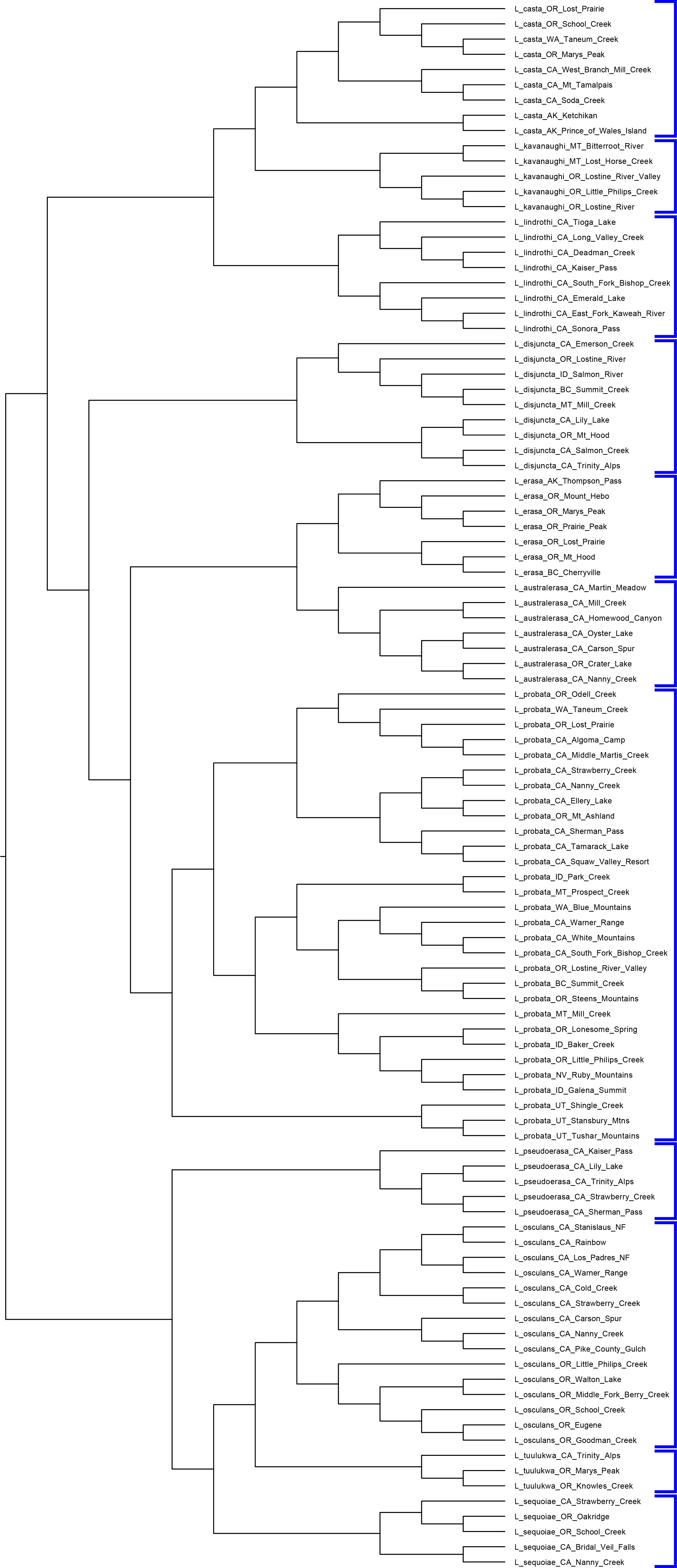
Figure: We cannot delimit populations for the entire data set simulatneously in BP&P due to the number of lineages. Instead, we decompose the analysis into a set of smaller analyses based on subtrees.
The set up for this set of analyses can be found at:
lionepha/02b-population-delimitation-subtrees
with each subdirectory containing a stand-alone analysis.
Collating Results of the Subtree Approach
Each of the subtree analysis now has the populations delimited under the MSC model. Having identified these population units across various subtrees, we now need to collate and pool them. DELINEATE helpfully provides a script for you to do this fairly robustly: delineate-bppsum. This script takes as its input two sets of files:
the “imap” files you provided to BP&P as input, which maps sequences to candidate population lineages
the output log of BP&P analyses (not the MCMC log), which provides a tree at the end with posterior probability of internal nodes indicated by labels
These files can be specified in any order, but must collectively span the entire analysis: the set of all candidate population names defined across all “imap” files must be equal to the set of all candidate population names found across all trees in all BP&P output log files.
In this example, we have all the independent subtree analyses packed away in subdirectories, “01”, “02”, etc.
Assuming we are in the BP&P analysis subdirectory, lionepha/02b-population-delimitation-subtrees, we could just type in all the paths:
delineate-bppsum \
    --imap    01/bpprun.input.imap.txt \
              02/bpprun.input.imap.txt \
              .
              .
              (etc.)
    --results 01/results.out.txt \
              02/results.out.txt \
              .
              .
              (etc.)
but because of judicious naming of the files, we can use some basic shell commands to generate the list of input files:
delineate-bppsum \
    --imap $(find . -name "*imap*") \
    --results $(find . -name "*out.txt")
Executing the above command results in:
[delineate-bppsum] 11 BPP 'imap' files specified
[delineate-bppsum] - Reading mapping file   1 of 11: ./00/bpprun.input.imap.txt
[delineate-bppsum]   - (13 lineages, 7 candidate populations)
[delineate-bppsum] - Reading mapping file   2 of 11: ./01/bpprun.input.imap.txt
[delineate-bppsum]   - (9 lineages, 9 candidate populations)
[delineate-bppsum] - Reading mapping file   3 of 11: ./02/bpprun.input.imap.txt
[delineate-bppsum]   - (10 lineages, 9 candidate populations)
[delineate-bppsum] - Reading mapping file   4 of 11: ./03/bpprun.input.imap.txt
[delineate-bppsum]   - (14 lineages, 7 candidate populations)
[delineate-bppsum] - Reading mapping file   5 of 11: ./04/bpprun.input.imap.txt
[delineate-bppsum]   - (12 lineages, 5 candidate populations)
[delineate-bppsum] - Reading mapping file   6 of 11: ./05/bpprun.input.imap.txt
[delineate-bppsum]   - (10 lineages, 8 candidate populations)
[delineate-bppsum] - Reading mapping file   7 of 11: ./06/bpprun.input.imap.txt
[delineate-bppsum]   - (16 lineages, 15 candidate populations)
[delineate-bppsum] - Reading mapping file   8 of 11: ./07/bpprun.input.imap.txt
[delineate-bppsum]   - (34 lineages, 30 candidate populations)
[delineate-bppsum] - Reading mapping file   9 of 11: ./08/bpprun.input.imap.txt
[delineate-bppsum]   - (9 lineages, 5 candidate populations)
[delineate-bppsum] - Reading mapping file  10 of 11: ./09/bpprun.input.imap.txt
[delineate-bppsum]   - (6 lineages, 5 candidate populations)
[delineate-bppsum] - Reading mapping file  11 of 11: ./10/bpprun.input.imap.txt
[delineate-bppsum]   - (10 lineages, 3 candidate populations)
[delineate-bppsum] 11 BPP output files specified
[delineate-bppsum] - Reading output file   1 of 11: ./00/results.out.txt
[delineate-bppsum]   - (7 candidate populations)
[delineate-bppsum] - Reading output file   2 of 11: ./01/results.out.txt
[delineate-bppsum]   - (9 candidate populations)
[delineate-bppsum] - Reading output file   3 of 11: ./02/results.out.txt
[delineate-bppsum]   - (9 candidate populations)
[delineate-bppsum] - Reading output file   4 of 11: ./03/results.out.txt
[delineate-bppsum]   - (7 candidate populations)
[delineate-bppsum] - Reading output file   5 of 11: ./04/results.out.txt
[delineate-bppsum]   - (5 candidate populations)
[delineate-bppsum] - Reading output file   6 of 11: ./05/results.out.txt
[delineate-bppsum]   - (8 candidate populations)
[delineate-bppsum] - Reading output file   7 of 11: ./06/results.out.txt
[delineate-bppsum]   - (15 candidate populations)
[delineate-bppsum] - Reading output file   8 of 11: ./07/results.out.txt
[delineate-bppsum]   - (30 candidate populations)
[delineate-bppsum] - Reading output file   9 of 11: ./08/results.out.txt
[delineate-bppsum]   - (5 candidate populations)
[delineate-bppsum] - Reading output file  10 of 11: ./09/results.out.txt
[delineate-bppsum]   - (5 candidate populations)
[delineate-bppsum] - Reading output file  11 of 11: ./10/results.out.txt
[delineate-bppsum]   - (3 candidate populations)
[delineate-bppsum] Posterior probability threshold of 0.50: 86 populations
[delineate-bppsum] Posterior probability threshold of 0.75: 72 populations
[delineate-bppsum] Posterior probability threshold of 0.90: 65 populations
[delineate-bppsum] Posterior probability threshold of 0.95: 59 populations
[delineate-bppsum] Posterior probability threshold of 1.00: 46 populations
and produces the following files:
coalescent-pops.sb2-traits.p050.txt
coalescent-pops.sb2-traits.p075.txt
coalescent-pops.sb2-traits.p090.txt
coalescent-pops.sb2-traits.p095.txt
coalescent-pops.sb2-traits.p100.txt
coalescent-pops.summary.csv
The population boundaries and identities of the various individuals are reported at different posterior probabilities (0.50, 0.75, 0.90, 0.95, and 1.00).
A comprehensive overview of all the identities under the different posterior probabilities is provided in the file: coalescent-pops.summary.csv.
The other files (ending with filenames “…sb2-traits.p0xx.txt”) are StarBeast2 “traits” files at each of those posterior probability thresholds.
These latter make setting up a StarBeast2 analysis to estimate an ultrametric phylogeny relating the population units delimited at each of the posterior probability thresholds very straightforward.
With the latter, do not be confused by the column header “species”!
Again, this is simply due to the misleading terminology adopted for the higher-level units of organization in StarBeast2 and most other programs that use the MSC.
What we are working with here are population units, some of which may also correspond to species while others may not.
This is abundantly clear by the fact that the 12 nominal species — established with both genomic as well as morphological data contributing toward an understanding of the system over a decade of the study — is split into 46 to 86 units (!) by the MSC analysis, depending on the posterior probability threshold we adopt for those units.
Interpreting these units as “species” is categorically and unconditionally wrong, and would represent a jettisoning of a basic understanding of speciation, systematics, and biology, due to a complete misunderstanding of the MSC model and misinterpretation of its results.
The MSC delimits populations, not species.
Note that where our candidate populations assignment have indeed turned out to be distinct population lineages under a particular posterior probability threshold, the original population label is retained (e.g., “L_australerasa_CA_Martin_Meadow” or “L_probata_WA_Blue_Mountains”).
In cases where multiple candidate population lineages have been “collapsed”, because there was insufficient signal for restriction of Wright-Fisher panmixia between them detected at a particular posterior probability threshold, they have been relabeled with synthetic labels (e.g. “coalescentpop001”, “coalescentpop002”, etc.). Thus, for example, we see that, in the setup to our BP&P analysies, we allowed for the possibility that L. erasa from Mary’s Peak, Mount Hebo, Mount Hood, and Prairie Peak might each be a distinct population:
sample |
BP&B Candidate Population (“Species”) |
|---|---|
L_erasa_OR_Marys_Peak_2575 |
L_erasa_OR_Marys_Peak |
L_erasa_OR_Marys_Peak_2586 |
L_erasa_OR_Marys_Peak |
L_erasa_OR_Marys_Peak_2615 |
L_erasa_OR_Marys_Peak |
L_erasa_OR_Marys_Peak_2616 |
L_erasa_OR_Marys_Peak |
L_erasa_OR_Mount_Hebo_3013 |
L_erasa_OR_Mount_Hebo |
L_erasa_OR_Mount_Hebo_3016 |
L_erasa_OR_Mount_Hebo |
L_erasa_OR_Mt_Hood_4144 |
L_erasa_OR_Mt_Hood |
L_erasa_OR_Prairie_Peak_2580 |
L_erasa_OR_Prairie_Peak |
Following the analysis, we see that at a 0.95 posterior probability threshold (see the “p095” column in 02b-population-delimitation-subtrees/coalescent-pops.summary.csv or 02b-population-delimitation-subtrees/coalescent-pops.sb2-traits.p095.txt) there was insufficient evidence to support four distinct populations here. Population boundaries between Marys Peak, Mount Hebo, and Prairie Peak was were not strong, and all individuals here were assigned to a single merged or collapsed population, “coalescentpop007”. Only the Mount Hood individuals were separated out to be delimited as a distinct population.
sample |
p095 |
|---|---|
L_erasa_OR_Marys_Peak_2575 |
coalescentpop007 |
L_erasa_OR_Marys_Peak_2586 |
coalescentpop007 |
L_erasa_OR_Marys_Peak_2615 |
coalescentpop007 |
L_erasa_OR_Marys_Peak_2616 |
coalescentpop007 |
L_erasa_OR_Mount_Hebo_3013 |
coalescentpop007 |
L_erasa_OR_Mount_Hebo_3016 |
coalescentpop007 |
L_erasa_OR_Mt_Hood_4144 |
L_erasa_OR_Mt_Hood |
L_erasa_OR_Prairie_Peak_2580 |
coalescentpop007 |
On the other hand, however, at the 0.50 posterior probability threshold, while the Mary’s Peak and Prairie Peak candidate population lineages were still collapsed into a single population (“coalescentpop004”), the Mount Hebo and Mount Hood individuals were each estimated to form a distinct population unto themselves (see the “p050” column in 02b-population-delimitation-subtrees/coalescent-pops.summary.csv or 02b-population-delimitation-subtrees/coalescent-pops.sb2-traits.p050.txt):
sample |
p050 |
|---|---|
L_erasa_OR_Marys_Peak_2575 |
coalescentpop004 |
L_erasa_OR_Marys_Peak_2586 |
coalescentpop004 |
L_erasa_OR_Marys_Peak_2615 |
coalescentpop004 |
L_erasa_OR_Marys_Peak_2616 |
coalescentpop004 |
L_erasa_OR_Mount_Hebo_3013 |
L_erasa_OR_Mount_Hebo |
L_erasa_OR_Mount_Hebo_3016 |
L_erasa_OR_Mount_Hebo |
L_erasa_OR_Mt_Hood_4144 |
L_erasa_OR_Mt_Hood |
L_erasa_OR_Prairie_Peak_2580 |
coalescentpop004 |
Going forward to the next stage of analysis, we have to decide the posterior probability threshold at which we want to determine our population units. For this example, we will (somewhat arbitrarily) decide on 0.95.
Stage II. Generating the (Multipopulation Coalescent, Ultrametric) Phylogeny of Populations
We use StarBeast2 to estimate an ultrametric phylogeny of population lineages.
We use the original set of alignments (found in lionepha/00-alignments) for as the input data for this, and a “traits” file that maps each of the sequence labels in the alignment to population identities assigned in the previous step.
For this exercise, we shall use population units that were delimited with 0.95 posterior probability, and the “traits” file corresponding to this is given by coalescent-pops.sb2-traits.p095.txt.
The analysis setup for the StarBeast2 run can be found in the lionepha/03-population-tree-estimation/ directory.
There are six StarBeast2 XML configuration files.
These all set up the same “species tree” analysis, the only difference being the name prefixes of the output files.
This is so that we can run multiple independent analyses, the sin qua non of MCMC best practices.
Again, we used a single strict clock model across all genes, and a HKY+G model of substitution. Each analysis was run for 400 million generations, with a sampling frequency of 400,000 generations. Thus, we obtained 1000 samples from the posterior from each of the six replicates. We can again use SumTrees to summarize the results with the following command:
$ sumtrees.py \
    -b 250 \
    -s mcct \
    -e mean-age \
    -l clear \
    --force-rooted \
    --suppress-annotations \
    -ro lionepha-p095-hkyg.mcct-mean-age.tree \
    *.species.trees
This will discard the first 250 of the 1000 samples from each replicate as burn-in, merge the results, and select the Maximum Clade Credibility Tree (MCCT) as the summary topology, with branch lengths set such that the internal node ages are the mean of the the corresponding node ages across all post-burnin samples. The result of this can be found here: lionepha/03-population-tree-estimation/lionepha-p095-hkyg.mcct-mean-age.tree.nex. This population-level phylogeny will be one of the two primary inputs to DELINEATE.
Stage III. Assignment of Known vs. Unknown Species Identities
We now inspect our phylogeny and determine a priori species assignments for as many population lineages as we can. These assignments will be made with reference to our integrative understanding of the system in conjunction with the evolutionary relationships between population lineages shown in the phylogeny.
There will be some population lineages for which the species identity is uncontroversial — i.e., they can be unambiguously assigned to known species (or even new ones) based on morphological evidence of individuals in that population. In the case of the “collapsed” populations (labeled “coalescentpop001”, “coalescentpop002”, etc.), we would need to examine all individuals in those units, and if any one of them can be definitely assigned to an independent species status based on systematic evidence (i.e., distinct species from all others in the system), then the entire population lineage would get assigned to a distinct species. The reasoning behind this is that, based on previous stages of the analysis using BP&P, we have already decided that all individuals in that population constitute a single cohesive population, so the species identity of any one individual in that lineage would necessarily be shared by all other individuals in the same lineage.
There will, of course, be population units for which we will not be able to confidentally assign to a distinct species status — either a known, existing one, or to a new one. These population lineages could be distinct species unto themselves, or could be populations of other species in the system (named or otherwise). These are the actual targets of delimitation — we would to determine whether or not the boundaries between them and other lineages are species boundaries or population boundaries.
The first set of population lineages — the ones for which we can confidently assign species identities, and, hence, boundaries — constitute our “constrained” lineages. We set them as constraints when we configure the DELINEATE analysis by setting their status to “1” in the constraints table. This can be seen with, for e.g., “coalescentpop001”, “coalescentpop002”, and “L_australerasa_CA_Martin_Meadow” in the example constraints file (04-species-delimitation/lionepha.run1.tsv; see below), which all have been assigned to “australerasa” (as can be seen in the “species” column), with the “status” set to 1. This will indicate to DELINEATE that the assignment of these populations to species is fixed, and we should not consider any partition that violates this.
lineage |
species |
status |
|---|---|---|
|
australerasa |
1 |
|
australerasa |
1 |
|
australerasa |
1 |
|
casta |
1 |
|
casta |
1 |
|
casta |
1 |
|
casta |
1 |
|
casta |
1 |
|
disjuncta |
1 |
|
disjuncta |
1 |
|
disjuncta |
1 |
|
disjuncta |
1 |
|
disjuncta |
1 |
|
erasa |
1 |
|
erasa |
1 |
|
erasa |
1 |
|
erasa |
1 |
|
erasa |
1 |
|
lindrothi |
1 |
|
lindrothi |
1 |
|
osculans |
1 |
|
osculans |
1 |
|
osculans |
1 |
|
osculans |
1 |
|
osculans |
1 |
|
osculans |
1 |
|
osculans |
1 |
|
probata |
1 |
|
probata |
1 |
|
probata |
1 |
|
probata |
1 |
|
probata |
1 |
|
probata |
1 |
|
probata |
1 |
|
probata |
1 |
|
probata |
1 |
|
probata |
1 |
|
probata |
1 |
|
probata |
1 |
|
probata |
1 |
|
probata |
1 |
|
pseudoerasa |
1 |
|
pseudoerasa |
1 |
|
sequoiae |
1 |
|
sequoiae |
1 |
Conversely, there remain a number of population lineages that we are not sure about (we are going to pretend, for the purposes of this exercise). These populations could be populations of existing species OR they could be independent species (either as a single lineage or clusters of lineages). These are the lineages that are the (remaining) primary focus of the species delimitation analysis. In the constraints table, we set the status of these lineages to “0”, indicating that we want the DELINEATE analysis to explore all possible partitions that vary in the species assignments of these populations. Note that we still have entries in the “species” field for this “unconstrained” lineages. This is purely for our own book-keeping and will be ignored entirely by DELINEATE. We could, in principle, replace them with any text or level them blank, and they will have no difference in the program running or output.
lineage |
species |
status |
|---|---|---|
|
? |
0 |
|
? |
0 |
|
? |
0 |
|
? |
0 |
|
? |
0 |
|
? |
0 |
|
? |
0 |
|
? |
0 |
|
? |
0 |
|
? |
0 |
|
? |
0 |
|
? |
0 |
|
? |
0 |
Stage IV. Delimitation of Species Units
We are now ready to run DELINEATE to carry out the species delimitation analysis. This will target the population lineages of unknown (“0”) status, and calculate the probabilities of all possible partitions that vary in their placement with respect to species identities. The full analytical setup can be found in the subdirectory 04-species-delimitation/. For input data, we will use the phylogeny obtained in Stage II (lionepha/03-population-tree-estimation/lionepha-p095-hkyg.mcct-mean-age.tree.nex) and the constraints table in Stage III (04-species-delimitation/lionepha.run1.tsv) as inputs to the program delineate-estimate. To execute the analysis, we run the following command:
delineate-estimate partitions \
    -P 0.99 \
    -t lionepha-p095-hkyg.mcct-mean-age.tree.nex \
    -c lionepha.run1.tsv
The “-P 0.99” flag says to only report the probabilities of all partitions that contribute collectively to over 0.99 of the probabilities. There could be thousands (or billions, depending on the number of unconstrained lineages you set) of other partitions in the 0.01 remaining tail that we choose to ignore to save disk space and time.
Note
Analysis Size and Computational Requirements
This analysis has 13 unconstrained lineages out of 56. The former (i.e., the number of unconstrained lineages) is the primary factor driving computational requirements, both in terms of time as well as memory: an analysis of 10,000 populations of which only 5 unconstrained will run faster (almost instantaneously) than one with 100 populations with 10 unconstrained. An analysis with 50 unconstrained lineages will probably never complete even with the most powerful computers thrown at it, regardless of how few or many the contrained lineages are. With this example of 13 unconstrained population lineages, we require 115 GB of computer memory and took about 35 mins to run on a fairly current (as of 2019) high-performance computing cluster. If you find that this might be too demanding for your hardware (especially the memory requirement), you can reduce the complexity of the analysis by “fixing” the status of a few more species to be constraints by changing some “0’s” to “1’s” in the status columns of the constraint file (04-species-delimitation/lionepha.run1.tsv).
The analysis will produce the following files:
lionepha.run1.delimitation-results.json
lionepha.run1.delimitation-results.trees
lionepha.run1.delimitation-results.trunc.trees
The first two are included in the example archive in compressed form: 04-species-delimitation/lionepha-delimitation-results.zip, while the last is given directly.
The JSON-format file (lionepha.run1.delimitation-results.json) lists some metadata about the analysis, followed by detailed description of all partitions considered. The partitions are listed in order of descending probability, i.e., with the partition of highest probability given first. Thus, the maximum likelihood estimate of the species delimitation is represented by the first partition listed. The second partition listed is the species delimitation of the next highest probability, and so on.
The tree file lionepha.run1.delimitation-results.trees consists of a set of trees, with one tree for each partition considered. The tree structure itself — the phylogeny, including both topology and the branch lengths — are identical across all trees. The only difference in the trees is the metadata markup of each tree, with annotations regarding species assignments of the tip (population) lineages. Each tree corresponds to the a partition listed in the JSON file, in the same order. Thus the trees illustrate the different partitions (and species assignments/boundaries of each partition), with the first tree representing the maximum likelihood estimate of the species delimitation, the second tree listed being the next most probable species delimitation and so on.
The third file lionepha.run1.delimitation-results.trunc.trees is also a tree file, but contains the just the first 10 trees from the primary results tree file (lionepha.run1.delimitation-results.trees) The results files can very large which may make viewing them challenging. To facilitate viewing/manipulating of the most probable results, we provide a smaller tree file with just the first 10 trees. As the the result entries (trees and partitions) are given in order of descending probability, the earlier results have a higher probability than the later ones, so truncating the tree file by selecting the first few like this will let you view the most probable results. Again, as with the primary tree file, the first listing in the results will have the highest probablity, and thus is MLE partition/tree.
Examination and Interpretation of the Results
The trees generated by DELINEATE have some special mark-up that will show up when opened in FigTree for visualization. For example, opening up the truncated trees result file (lionepha.run1.delimitation-results.trunc.trees) in FigTree and viewing the first tree, i.e. the maximum likelihood species delimitation shows the following:
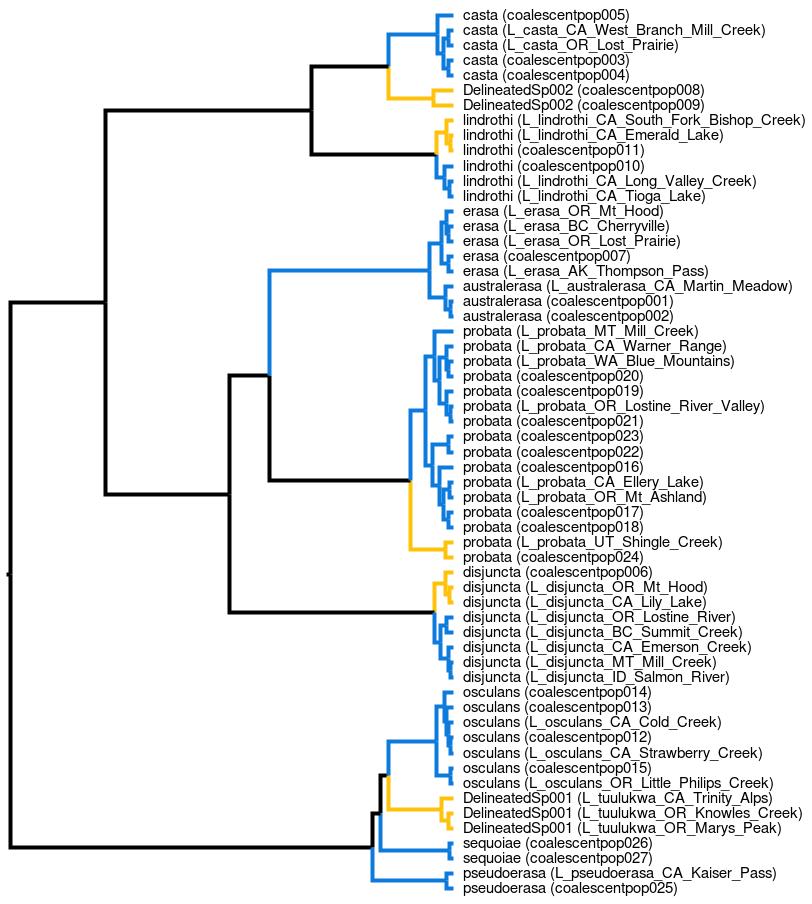
The branches painted in blue (▆) represent the constrained population lineages, i.e., lineages with a fixed species assignment. The branches painted in ochre (▆), on the other hand, represent the unconstrained population lineages, i.e., lineages with unknown species identity and whose species membership was allowed to vary. Furthermore the lineage labels are in a special format, showing the species assignment followed by the actual population label in parenthesis.
We interpret the results as follows:
Lineages |
Species Delimitation |
Explanation |
|---|---|---|
|
DelineatedSp002 |
Group together in the same NEW and unnamed species, labeled “DelineatedSp002”. That is, the boundaries between these two lineages on the one hand, and all other lineages on the other, are species boundaries, not population. |
|
lindrothi |
Group together as populations that are part of a pre-defined species, “L. lindorothi”. That is, the boundaries between these three lineages on the one hand, and all other lindrothi lineages on the other, are (just) population boundaries, not species. |
|
probata |
Group together as populations that are part of a pre-defined species, “L. probata”. That is, the boundaries between these two lineages on the one hand, and all other probata lineages on the other, are (just) population boundaries, not species. |
|
disjuncta |
Group together as populations that are part of a pre-defined species, “L. disjuncta”. That is, the boundaries between these three lineages on the one hand, and all other disjuncta lineages on the other, are (just) population boundaries, not species. |
|
DelineatedSp001 |
Group together in the same NEW and unnamed species, labeled “DelineatedSp001”. That is, the boundaries between these three lineages on the one hand, and all other lineages on the other, are species boundaries, not population. |
Conferring with the reference alpha taxonomy as worked out by Maddison and Poul (2020), we see that these are perfectly concordant. The “DelineatedSp001” populations all collectively corresponded to the distinct species L. tuulukwa and “DelineatedSp002” populations all collectively corresponded to the distinct species L. kavanaughi. At the same time, the remaining unconstrained population lineages in our example indeed were referred to probata, lindrothi, and disjuncta species.